The Genome as a History Book:How PSMC Unveils Population History from a Single Genome

Yufan Han (Larry)•May 7, 2025

Human DNA is not just a blueprint for growth and development, but also a detailed logbook recording the collective journey of our ancestors. It contains subtle clues about whether ancient populations flourished, struggled for survival, or migrated. This raises a core question: Can we estimate the size of our ancestral populations thousands or even millions of years ago by analyzing the DNA of just one modern individual?

Since the turn of this century, bioinformatics has flourished, with scientists creatively inventing numerous tools to decipher genomic history. Among these, the Pairwise Sequentially Markovian Coalescent (PSMC) algorithm is undoubtedly a landmark achievement. Proposed by Heng Li and Richard Durbin in 2011, PSMC's magic lies in its ability to reconstruct the dynamic history of effective population size ($N_e$) of its host population over long periods, using only the diploid genome sequence of a single individual. This "seeing the many from the few" capability starkly contrasts with many methods that require large numbers of individual samples.

Since its inception, PSMC has been widely used to study the population histories of humans, archaic hominins (like Neanderthals and Denisovans), various animals (such as ancient horses, wolves, mammoths, birds, bears, apes, pandas), and even plants, proving particularly adept at revealing ancient population dynamics. It can also help infer speciation times and estimate key evolutionary parameters like mutation rates.

This article will delve into the PSMC algorithm. We will first introduce the core biological concepts behind it – Coalescent Theory and genetic recombination – then explain how PSMC cleverly uses Hidden Markov Models (HMMs) to extract historical information from genome sequences, showcase some of its interesting discoveries, discuss its limitations, and look ahead to future developments in the field.

The Genome: A Historical Document Written by Recombination and Coalescence

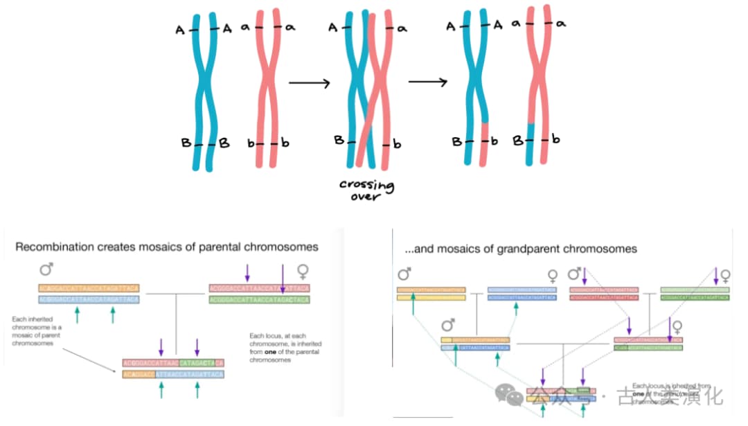
Imagine our genome. For most chromosomes (except sex chromosomes), we inherit one set from each parent. However, due to genetic recombination occurring during generational transmission, the chromosomes we inherit from our parents are not complete "paternal" or "maternal" versions but are "mosaic segments" pieced together from different fragments originating from earlier ancestors. This means that along the same chromosome, different segments can have vastly different ancestors and historical narratives.

Caption for the image

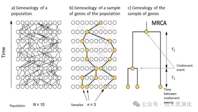
To understand the history of these segments, we need to introduce Coalescent Theory. Unlike the traditional perspective of looking from ancestors to descendants, coalescent theory takes a "looking back in time" approach. It traces the lineages of alleles (different versions of a gene) in a sample, observing how they gradually merge (coalesce) in past generations, eventually converging to a common ancestor. For any pair of lineages, the point in time when they meet their common ancestor is called the Time to Most Recent Common Ancestor (TMRCA).

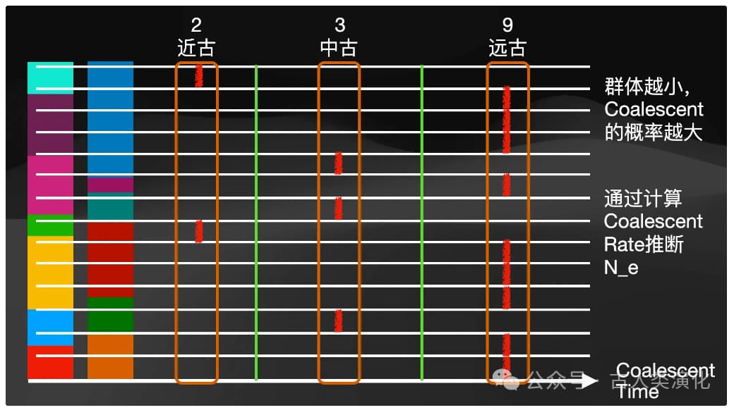
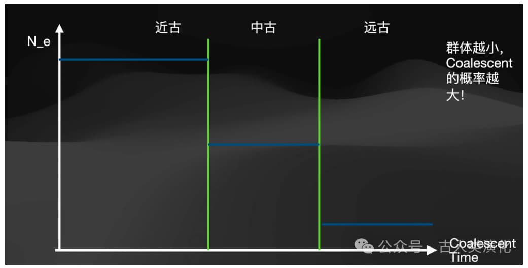
The core of coalescent theory lies in its revelation of the profound connection between the rate of lineage coalescence and the effective population size ($N_e$). Effective population size can be understood as the size of an idealized, randomly mating population that would experience the same amount of genetic drift as the actual population. Simply put:

• In a small effective population, individuals are more closely related, and any two gene lineages are more likely to find a common ancestor in the recent past. Thus, coalescence occurs faster, and the average TMRCA is shorter.
• In a large effective population, individuals are relatively distantly related, and lineages need to be traced back further in time to find a common ancestor. Thus, coalescence occurs more slowly, and the average TMRCA is longer.

This inverse relationship is fundamental to inferring population history from genomic information. Theoretically, the probability of two lineages coalescing is proportional to $1/(2N_e)$.

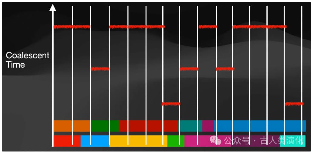
However, coalescent theory tells us that the coalescence rate is related to population size, meaning we need to observe multiple coalescence events to infer history. Yet, PSMC uses only the genome of a single individual (i.e., two sets of homologous chromosomes). So, how does it obtain enough information to infer the history of an entire population? The answer lies in the power of genetic recombination. It is precisely because recombination cuts and reshuffles an individual's two chromosomes into countless segments with different ancestral histories that the TMRCAs between corresponding segments on these two chromosomes vary along the genome. These different TMRCA values reflect the effective population sizes at the times they coalesced (i.e., at different historical time points). Therefore, by analyzing the distribution and variation of TMRCAs across a single individual's genome, PSMC effectively samples a large number of independent pairwise coalescence events from the past. Genetic recombination cleverly transforms a diploid genome into a rich data source for studying population history, which is key to how PSMC can infer the "whole" from the "one."

Unveiling Hidden History: The Magic of Hidden Markov Models (HMMs)

To infer the hidden TMRCA history (which we cannot see) from the genome sequence (which we can see), PSMC employs a powerful statistical tool – the Hidden Markov Model (HMM).

We can understand HMMs with a simple analogy. Suppose you want to know the weather on a given day (sunny or rainy), but you are confined to a windowless room. The only thing you can observe is how much ice cream people outside ate that day. In this example:

• Hidden States: The true situation you cannot directly observe, i.e., the weather (sunny/rainy).
• Observations / Emissions: The data you can see, generated by the hidden states, i.e., ice cream sales (e.g., 1, 2, or 3 units).
• Transition Probabilities: The likelihood of transitioning between hidden states. For example, what is the probability that if it's sunny today, it will still be sunny tomorrow? What is the probability it will turn rainy?
• Emission Probabilities: The likelihood of producing a specific observation given a certain hidden state. For example, if it's sunny, what is the probability people eat 3 ice creams? If it's rainy, what is the probability they eat 1?

The core idea of an HMM is to infer the most likely sequence of hidden states (the actual weather over those days) by analyzing a sequence of observations (ice cream sales over several days), combined with our knowledge (or estimates) of transition probabilities (patterns of weather change) and emission probabilities (how weather affects ice cream consumption).

HMMs also incorporate an important Markov Property: the current state depends only on the immediately preceding state, not on earlier states. Just like predicting tomorrow's weather only requires knowing today's weather. In genomic analysis, this means the TMRCA at one position is primarily influenced by the TMRCA of the immediately preceding position and whether recombination occurred between them. Although this is an approximation for genomes (known as the SMC approximation), it has proven very effective in practice.

How PSMC Works: The HMM on the Genome

Now, let's map the HMM concepts specifically to the PSMC algorithm:

As shown in the figure, HMM can be used to estimate the discretized TMRCA for each genomic region.

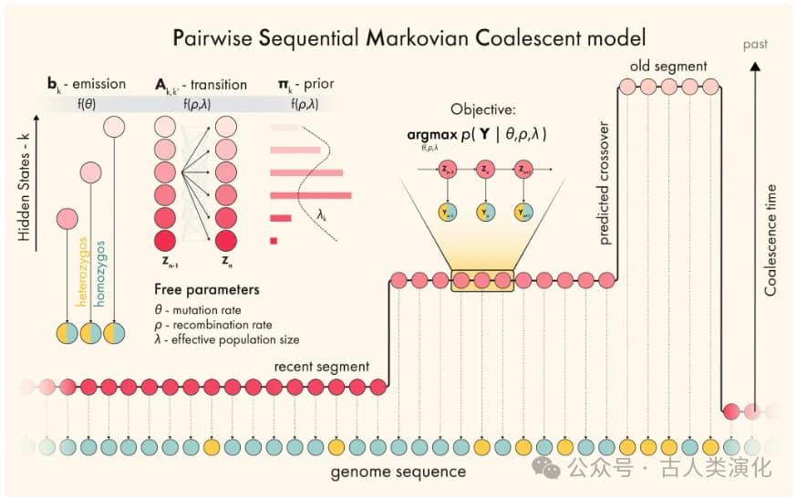
• Hidden States: Discretized TMRCA. Since TMRCA is a continuous time value and standard HMMs require discrete states, PSMC divides time backwards into multiple (e.g., 32 or 64) non-overlapping time intervals. Each interval represents a hidden state, indicating that the common ancestor of the two lineages at a genomic locus falls within this time period.
• Observations (Emissions): Local heterozygosity. PSMC divides the genome into many small windows (e.g., 100 bp). Within each window, the algorithm checks if the two chromosomes of the diploid individual differ at any site (i.e., a heterozygous site). If at least one difference exists, the window is marked as "heterozygous" (e.g., denoted by 'K' or '1'); if no differences exist, it's marked as "homozygous" (e.g., 'T' or '0'). Thus, the entire genome is converted into a sequence of 0s and 1s (or Ts and Ks) serving as input for the HMM.
• Emission Probabilities: The probability of observing heterozygosity given a TMRCA state. This probability primarily depends on two factors: the hidden TMRCA state and the mutation rate ($\mu$). The longer the TMRCA, the longer the two lineages have been separated, allowing more opportunities for mutations to accumulate, thus increasing the probability of observing a heterozygous site in that window. In the PSMC model, this probability is typically related to $2\mu t$ (where $t$ is the TMRCA). More precisely, it's related to the population mutation rate $\theta =4N_e\mu$.
• Transition Probabilities: The probability of transitioning from one TMRCA state to another. This is primarily determined by the recombination rate ($\rho$). As the algorithm moves from one window to the next along the chromosome, if an ancestral recombination event occurred between these two windows, the TMRCA of the next window may differ from the previous one, leading to a transition in the hidden state. The probability of transition depends not only on the recombination rate but also on the population history at the time of recombination (which affects the coalescence probability of the new lineages post-recombination).

The PSMC workflow can be summarized as:

1. Input: Process the individual's diploid genome sequence into a sequence representing heterozygous/homozygous states (e.g., one marker per 100 bp).
2. HMM Computation: The algorithm "walks" along the chromosome, using HMM computation methods (like the forward-backward algorithm), combined with the observed heterozygous/homozygous sequence, preset (or estimated) mutation and recombination rates, and transition probabilities between states, to calculate the likelihood of being in each discrete TMRCA state at every genomic position.
3. TMRCA Distribution Estimation: Integrate information from the entire genome to obtain a global TMRCA distribution, i.e., the proportion of genomic segments whose common ancestors fall into each respective time interval.

4. $N_e$ History Inference: (Metaphorically) "rotate" the TMRCA distribution (from step 3). Using the core relationship from coalescent theory mentioned earlier—that the coalescence rate (reflected in the TMRCA distribution) is inversely proportional to effective population size ($N_e$)—convert the inferred TMRCA distribution into estimates of $N_e$ for different past time periods.

PSMC results on simulated data: the blue line is the true history, and the red line is the PSMC-estimated effective population size history.

5. Output: The final result is usually presented as a plot with logarithmic time on the x-axis (past to the left, present to the right) and logarithmic effective population size ($N_e$) on the y-axis. The curve depicts changes in population size over time. The algorithm also provides estimates of the overall average (scaled) mutation rate ${\theta }_0$ and recombination rate. It's important to note that the output time and population size are scaled; users need to provide the actual per-generation mutation rate ($\mu$) and generation time ($g$) to convert them into absolute units (like years, number of individuals).

PSMC results on simulated data: blue line is the true history, red line is the PSMC-estimated effective population size history.

When understanding PSMC's workings, we must address a key issue: the dilemma of time discretization. The standard HMM framework requires discrete hidden states, but the TMRCA that PSMC aims to infer is inherently a continuous time value. Therefore, PSMC must divide the continuous time axis into discrete intervals (bins). This discretization is an approximation and inevitably introduces some problems. Firstly, it can lead to bias, as true TMRCAs might fall near the boundaries of two intervals, or the chosen binning scheme might not accurately reflect the true TMRCA distribution pattern, potentially creating artificial fluctuations at interval boundaries. Secondly, the computational complexity of HMM algorithms is typically related to the number of states (i.e., the number of time intervals, $T$), being at least $O(T)$ or even $O(T^2)$. This means increasing the number of time intervals to improve resolution significantly increases computational cost. Thus, time discretization is not only a potential source of error in the PSMC model but also a bottleneck for its computational efficiency. Recognizing this is crucial for understanding the motivation behind the development of subsequent algorithms (like Gamma-SMC, XSMC) that attempt to avoid discretization.

What PSMC Reveals: A Journey Through Population History Across Time

PSMC's output plot provides a window into the past. The x-axis represents time (usually on a logarithmic scale, with older times to the left), and the y-axis represents effective population size ($N_e$) (also often on a logarithmic scale). An upward sloping curve indicates population expansion, while a downward slope signifies population contraction or a bottleneck. In its initial applications, PSMC painted a grand picture of human prehistory:

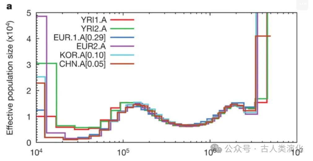
• All modern human groups (African, European, Asian) shared very similar population histories before about 150,000-200,000 years ago, with relatively large effective population sizes.
• African populations (like the Yoruba) also experienced a bottleneck, but it was less severe and they recovered earlier.
• Between approximately 60,000 and 250,000 years ago, the effective population sizes of all groups appear unusually high, possibly reflecting ancient population substructure at the time (i.e., populations were not completely randomly mating).
• PSMC results also suggested that the genetic divergence of modern humans might have begun as early as 100,000-120,000 years ago, but significant gene flow between different groups likely continued until about 20,000-40,000 years ago before largely ceasing. (This view on divergence times and gene flow events is subject to ongoing debate and knowledge refinement).

PSMC's Assumptions and Limitations

Although PSMC is powerful, its use and interpretation of results require caution, as it is built on a series of assumptions and has inherent limitations.

The "Random Mating" Assumption

PSMC's core assumption is that the analyzed individual comes from a single, large, panmictic population (i.e., individuals within it mate completely randomly). However, growing research indicates that the history of many species (including humans) is not so simple, often involving population structure, such as subpopulation divergence, migration restrictions, or ancient admixture. In such cases, the curve inferred by PSMC actually reflects the Inverse Instantaneous Coalescence Rate (IICR), rather than purely the effective population size ($N_e$). When population structure exists, lineages from different subpopulations take longer to coalesce, artificially elongating the TMRCA distribution and making the IICR appear larger than the true $N_e$. PSMC can misinterpret this structure-induced delay in coalescence as a historically larger population or misread concentrated coalescence times as population bottlenecks. Therefore, when interpreting PSMC results, one must be wary of the confounding effects of population structure. A seemingly severe bottleneck might not be a true population crash but could reflect ancient subpopulation divergence or reduced gene flow.

Limitations in Temporal Resolution

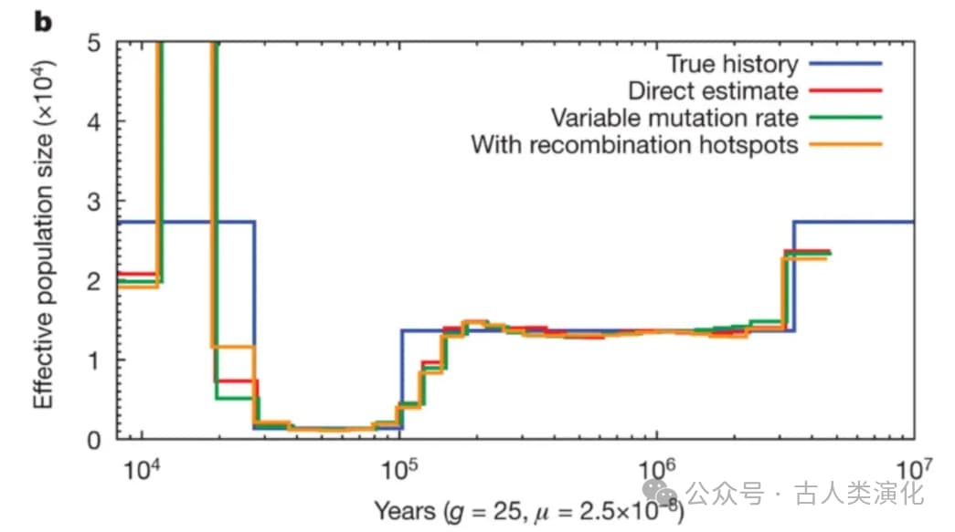
PSMC has limited ability to infer very recent history (e.g., within the last 20,000-30,000 years for humans). This is because, over such short periods, relatively few recombination events occur between the two strands of a diploid genome, insufficient to generate enough TMRCA variation to accurately resolve recent population dynamics. Similarly, for very ancient history (e.g., beyond 1-3 million years for humans), its inference power diminishes due to potential mutation saturation or loss of recombination information. Furthermore, PSMC tends to smooth out sudden, drastic changes in population size (like instantaneous bottlenecks or expansions), making it difficult to capture their abrupt nature.

The Influence of Natural Selection

PSMC assumes that the analyzed genomic regions are neutral, i.e., not under the influence of natural selection. However, natural selection (such as selective sweeps driven by positive selection, or background selection (BGS) caused by negative selection) can alter local patterns of genetic diversity, thereby interfering with PSMC's inferences. Background selection, in particular, reduces the effective population size of linked regions, causing PSMC to erroneously infer population contractions or bottlenecks, especially in recent times.

Recognizing these limitations of PSMC is crucial for understanding the development of subsequent methods. It can be said that each weakness of PSMC has spurred the creation of new algorithms. For instance, MSMC emerged to improve resolution for recent history and utilize more sample information. SMC++ was developed to handle larger sample sizes and integrate allele frequency information. PSMC+ was proposed to correct biases introduced by natural selection. Methods like cobraa, IS-MSMC, and MSMC-IM were designed to more accurately model population structure and admixture. To overcome the problem of time discretization and improve computational efficiency, methods like Gamma-SMC, XSMC, and diCal adopted different strategies. Thus, the history of SMC-like methods after PSMC clearly demonstrates the iterative process of "problem identification → problem-solving" in scientific research.

Conclusion

PSMC and its successor methods have undoubtedly provided unprecedentedly powerful tools for extracting population history information from genome sequences, profoundly changing our understanding of life's evolution. They enable us to quantify past population fluctuations and link them to macro-level processes such as climate change, geographical events, and speciation.

However, like all scientific tools, these model-based inference methods are not infallible. They rely on specific mathematical assumptions (such as the Markov property, specific recombination and coalescence models) and biological assumptions (such as panmixia, neutral evolution). When these assumptions deviate from reality, the interpretation of results requires extra caution. Factors like population structure, natural selection, and data quality can all interfere with inferences. Therefore, in practical applications, researchers often need to combine multiple analytical methods and utilize evidence from different sources (such as archaeology, paleoclimatology) to make comprehensive judgments.

Excitingly, this field is still rapidly evolving. New algorithms are constantly emerging, becoming more complex, scalable, and robust in simulating various biological realities with greater fidelity. From addressing biases due to selection and structure, to integrating more data types, and enhancing computational efficiency and inference accuracy, researchers are tirelessly working to more accurately and comprehensively decipher the information encoded within the DNA double helix in our cell nuclei—information about the evolution of life and our own origins. The journey of reading this genomic history book is far from over.